The abstract <Data Table> class (shown conceptually in figure 3-1) defines an N dimensional array of data cells. The dimension N is determined by the number of ordered <Axis> objects aggregated as components by a given <Data Table>. Each <Axis> component determines the number of cell ranks in its coordinate dimension. Consequently, a <Data Table> with two axes of size m and n will have m * n cells. A <Data Table> also aggregates an ordered list of <Table Property Description> components. This list constitutes the signature of the table. Each cell contains as many data items (properties) as there are <Table Property Description> components in the signature. These <Table Property Description> components describe each data item: its meaning, the units of measure, and the storage type (EDCS_Integer, EDCS_Long_Float, and so on). However, the dimensions and signature do not fully describe the intended meaning of the <Data Table>. For that, a <Classification Data> instance is provided as a component of each <Data Table> instance.
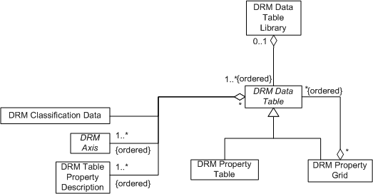
NOTE: We use the term "conceptual diagram" to denote those parts of the SEDRIS Data Representation Model class diagram that are relevant to the concept under discussion. See Appendix A of Part 4, Volume 17: SEDRIS Reference Manual for full class diagrams. Also note that the conceptual diagrams display class fields for convenience.
The <Classification Data> identifies the nature of the table and its likely signature. (See Part 4, Volume 10: EDCS Reference Manual). During SEDRIS transmittal data extraction, this information can be used in search filters. (See Part 4, Volume 13: How to Extract Data from SEDRIS Transmittals).
The abstract diagram shown in Figure 3-1 will be refined in later sections. For example, several classes are derived from the abstract <Data Table> class: <Property Grid>, <Property Table>, and <Mesh Face Table>. This conceptual diagram will change in later sections to reflect these and other refinements.
It is important to note that once data has been stored in a <Data Table> instance, the data type and number of axes cannot be changed without invalidating the data stored in the table. If the structure must be changed, it is typically best to create a new <Data Table> instance with the desired structure, then migrate existing data from the old <Data Table> instance to the new one.
The <Data Table> class defines an array of data cells. In general, these cells have no meaningful location in space. If the cells do correspond to gridded locations in space, then some of the axes must be spatial. The <Property Grid> class is used for <Data Tables> that include at least one spatial axis. As discussed in Section 2, we must
- specify the spatial reference frame that preserves the "griddedness" of the cells,
- orient and locate one cell in space, and
- identify which <Axis> components are the spatial axes.
In an analog to a <Geometry Model> instance, which is referenced at a spatial location using a <Geometry Model Instance> that provides a <Transformation>, the DRM provides the <Property Grid Hook Point> class, a subclass of <Geometry Hierarchy>, to tie a <Property Grid> instance to a spatial location within the geometric context in which it is to be referenced. A <Property Grid Hook Point> instance specifies the spatial location as a <Location> component, while a <Property Grid> instance specifies which of its cells corresponds to that location.
The conceptual diagram is presented in Figure 3-2.
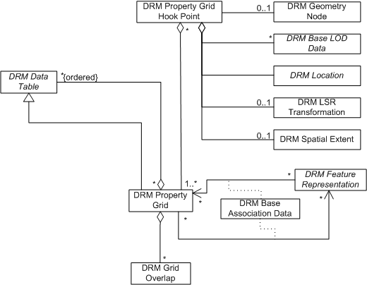
<Property Grid> has several fields in addition to those inherited from <Data Table>, namely, spatial_axes_count, location_index, srf_context_info, and data_present.
Note that a <Property Grid> instance specifies its own SRF. This may or may not match the SRF in which the <Property Grid> is instanced. The spatial_axes_count shall correspond to the <Property Grid>'s own SRF, rather than that of whatever context instances the <Property Grid>. The spatial_axes_count field specifies which of the ordered <Axis> components of a given <Property Grid> are spatial, in accordance with the <<Spatial Axis Constraints>>.
For example, if a <Property Grid> specifies its srf_context_info as Augmented Mercator (AM), then there can be no more than one "x" axis, "y" axis, or elevation / "z" axis.
The cell corresponding to the <Property Grid Hook Point>'s <Location> has indices on the 3 or fewer spatial axes specified by location_index[3]. Notice that location_index is not required to specify a point that actually lies within the boundaries of the grid. This allows several neighbouring <Property Grid> instances to be offset from the same <Property Grid Hook Point>, if desired.
In relation to Section 1, <Property Grid Hook Point> provides (1'), the location of one reference cell. The srf_info field generalizes requirements (2'), (3), and (6), while the <Axis> and <Table Property Description> components correspond to (9) and (7).
Note that a <Property Grid> can aggregate other <Data Table> instances as ordered components. This allows a cell signature item to reference (by index) a component <Property Grid> or <Property Table>, as well as a <Property Grid> or <Property Table> in a <Data Table Library>. A referenced <Property Grid> is located using the spatial location of the cell that references it as the location corresponding to its location_index. The topic of nested <Property Grid> instances will be treated in more detail below.
The <Property Table> class is used to store tabular data that requires no spatial axes (such data is stored in <Property Grid> instances). A <Property Table> may aggregate other <Property Table> instances as ordered components, which are then referenced in the cells of the table by component index. <Property Grid> instances cannot be referenced in this way by a <Property Table>, because the <Property Table> provides no spatial location to tie the <Property Grid>'s location_index to the instancing spatial reference frame.
Figure 3-3 is the conceptual diagram for the <Property Table> class.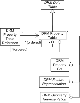
The <Mesh Face Table> class is used exclusively with the <Finite Element Mesh> class, which is discussed in section 4.
Attributed data is used throughout the DRM. To fully specify a data value, its meaning and storage type are required; if it is a numeric value, a scaled unit of measure is also required. Consequently, the data signature of a <Data Table> cell needs this information for each data item.
The abstract class <Property> abstracts the common fields for property values and signature items. It specifies the meaning of the property being represented by an SE_Element_Type field, meaning, and specifies the corresponding scaled unit of measure as value_unit and value_scale. An SE_Element_Type field value may represent an SE_Index_Code, SE_Variable_Code, or an EDCS_Attribute_Code (EAC). EACs are by far the most common. EDCS Attribute Codes, Unit Codes, and Scale Codes are specified as part of the Environmental Data Coding Specification (EDCS); see Part 4, Volume 10 EDCS Reference Manual for details.
<Property> has three concrete subclasses: <Property Value>, <Table Property Description>, and <Property Description>, each of which serves a slightly different purpose and provides different functionality.
<Property Value> serves to specify a single data value, with its meaning and unit of measure. Consequently, it has a value field, in addition to the fields inherited from <Property>. The value is a tagged union, wherein the tag specifies the storage type, and the union member stores the value itself. A <Property Value> may also have <Property Characteristic> components, but these are more commonly used by the other subclasses of <Property>, and are discussed later in this section.
<Table Property Description> represents a signature item in a <Data Table>. Since the values are stored in the cells of a <Data Table> instance, it does not have a value field. On the other hand, all the cells corresponding to a given <Table Property Description> have the same storage type, so the most practical approach is to record the storage type for a given signature item once, in the fields of the <Table Property Description>, rather than replicating it for each cell corresponding to that signature item. Consequently, <Table Property Description> has a value_type field, in addition to the fields inherited from <Property>.
As noted in previous sections of this document, a <Data Table> cell may reference other <Data Table> instances, if they are components of the referencing <Data Table> instance or if they reside in a <Data Table Library>. To reference another table in this manner, the meaning field of the applicable <Table Property Description> in the referencing table is set to the appropriate SE_Index_Code, while each of the referencing table's cells for that signature item contains an index number. Consider a reference to the Kth ordered component <Data Table>. The meaning of the <Table Property Description> is { SE_ELEMTYPCOD_INDEX, SE_IDXCODE_DATA_TABLE_COMPONENT }, while the referencing cell contains the appropriate index value. Other index code meanings are handled in a similar fashion.
If the DRM allowed only one signature item in any given <Data Table> instance to reference a component or library table, then the index value would simply be the index of the table within the specified list. However, the DRM grants more flexibility than that. Note that a <Table Property Description> contains a field that has not been discussed up to this point: component_data_table_ecc, and an optional ordered list of <Property Value> components that exist to qualify the component_data_table_ecc, if one is specified. This allows the provider of a <Data Table> to reference, not the Kth component <Data Table>, but the jth component <Data Table> that matches the given qualified ECC.
As noted earlier in this section, sometimes a given signature item requires the specification of special values, such as sentinel values, or the data provider wishes to provide extra information, such as maximum value, minimum value, or measurement error.
<Property Description> serves to provide context within the scope of an <Aggregate Feature> or <Aggregate Geometry> for all <Property Value> instances falling within its scope, in one of two ways.
A <Property Description> may have qualifying <Property Value> components, which then apply to all <Property Value> instances within that scope that have matching meaning field values. For example, in an <Aggregate Geometry> containing many <Polygon> instances that specify different emissivity values, the aggregate can contain a single <Property Description> component specifying the electromagnetic band.
A <Property Description> may also have <Property Characteristic> components, specifying special information, such as maximum value or minimum value.
| 3.6.1 | The <Axis> Class |
|---|---|
The <Axis> class abstracts the common characteristics of its concrete subclasses; each <Axis> instance specifies a meaning (the axis_type, a scaled unit of measure (the axis_unit and axis_scale), and a count for the number of tic marks on the axis (the axis_value_count). | |
| 3.6.2 | The <Regular Axis> Class |
The <Regular Axis> class is used to specify numerical axes that have a constant spacing between the axis values (which are called tick marks). To specify these regularly spaced values, a <Regular Axis> needs to specify the starting value (its first_value field), the type of spacing being used (spacing_type), and the spacing itself ( spacing). The notion of equal spacing applies to both arithmetic and geometric spacing. If SE_SPACTYP_ARITHMETIC is specified, then the kth tick mark value is tick(k) = first_value + (k * spacing) If SE_SPACTYP_GEOMETRIC is specified, then the kth tick mark value is tick(k) = first_value * (spacingK) When a <Regular Axis> is used to represent a continuous value, such as a spatial coordinate, it is often useful to interpolate between axis tick marks in order to estimate data values for points that fall between grid points. For example, a data consumer may wish to resample the data in a <Property Grid> to fit a grid specified in a different spatial reference frame. However, the appropriate interpolation method is data dependent. Differing interpolation techniques produce incompatible results, which is contrary to SEDRIS' interoperability objectives. Even simplistic techniques, such as linear interpolation, are inappropriate for certain kinds of environmental data, for instance, some kinds of oceanographic data. To allow a data consumer to perform data interpolation correctly, for the purpose of resampling or any other reason, the necessary interpolation method shall be provided with the data, by means of the interpolation_type field of <Regular Axis>. The currently supported interpolation methods are specified by the enumerants of SE_Interpolation_Type. Data specified by non-spatial <Axis> instances may never require interpolation. In these cases, the data provider specifies SE_INTERPOLATION_TYP_DISALLOWED. Spatial axes are not permitted to disallow interpolation, although a data provider may indicate that a preferred interpolation method is not supplied. | |
| 3.6.3 | The <Irregular Axis> Class |
The essential difference between <Regular Axis> and <Irregular Axis> - that one uses regular spacing to specify its tick marks and the other does not - results in certain differences in the fields required by <Irregular Axis>. Since the spacing is not regular, neither a spacing value nor a spacing type is specified, and the tick marks are not left to be computed by the consumer; instead, the tick mark values are provided explicitly in the axis_value_array field of the class, the size of which is specified by axis_value_count. Note that the <Irregular Axis> class has an interpolation_type field just as the <Regular Axis> class does. If a <Irregular Axis> is used to represent a spatial <Axis> within a <Property Grid>, the values within axis_value_array are all offsets from the location corresponding to the location_index of the grid. That is, if the axis is the ith spatial axis of a grid, and a is the corresponding coordinate value of the location cell, then the kth tick coordinate value is
a + axis_value_array[k]
where k ranges from zero (0) to axis_value_count -1. In particular, there is no offset at the location cell tick
axis_value_array[location_index[i]] = 0.0
Because there are only axis_value_count - 1 intervals determined by this array, there is no "last" interval. In particular, the non-existent last interval has neither middle nor upper point, so axis alignment for an <Irregular Axis> is always SE_AXALGN_LOWER. As specified by the <<General Axis Constraints>> constraint, the values in axis_value_array shall be unique and monotonic to avoid ambiguity. | |
| 3.6.4 | The <Enumeration Axis> Class |
An <Enumeration Axis> instance is contrained to specify an axis_type corresponding to an EDCS Attribute Code that is bound to a set of EDCS_Enumerant_Codes, from which its tick marks are supplied as its axis_value_array. | |
| 3.6.5 | The <Interval Axis> Class |
An <Interval Axis> instance specifies an interval for each axis value. Each entry in its axis_interval_value_array field is required to be bound to an interval storage type. |
| 3.7.1 | Overview | ||||||||||||||||||||||||||||||||||||||||||||||||||||||||||||
|---|---|---|---|---|---|---|---|---|---|---|---|---|---|---|---|---|---|---|---|---|---|---|---|---|---|---|---|---|---|---|---|---|---|---|---|---|---|---|---|---|---|---|---|---|---|---|---|---|---|---|---|---|---|---|---|---|---|---|---|---|---|
Several classes other than those already discussed either used or are needed by the <Data Table> class or one of its subclasses. The <Finite Element Mesh> class will be discussed in section 6, while the others are discussed in the remainder of this section. | |||||||||||||||||||||||||||||||||||||||||||||||||||||||||||||
| 3.7.2 | The <Data Table Library> Class | ||||||||||||||||||||||||||||||||||||||||||||||||||||||||||||
<Data Table Library> is a subclass of <Library> that exists to organize <Data Table> instances so that they can be referenced by objects within a transmittal. This is useful when two or more objects reference the same <Data Table> instance, because placing it in a <Data Table Library> makes the reuse of the instance explicit (c.f. Object Reuse in Part 4, Volume 14: How to Produce SEDRIS Transmittals). Note that while syntactically, any <Data Table> instance may belong to a <Data Table Library>, semantically <Mesh Face Table> instances do not do so, since this would violate the <<Constraints On Components>> constraint. By contrast, any <Property Table> that is referenced by a <Property Table Reference> (see below) is required to belong to a <Data Table Library>. | |||||||||||||||||||||||||||||||||||||||||||||||||||||||||||||
| 3.7.3 | The <Property Table Reference> Class | ||||||||||||||||||||||||||||||||||||||||||||||||||||||||||||
The <Property Table Reference> class exists to provide a mechanism for a <Feature Representation> or >Geometry Representation> instance to reference an N-1 dimensional 'slice' or (hyper-plane) of a N-dimensional <Property Table> residing in a <Data Table Library>. A <Property Table Reference> can be thought of as a "lookup entry" into a particular <Property Table> row or column, and has 2 fields: axis_type and index_on_axis. The axis_type field matches 1 <Axis> of the target <Property Table>, while the index_on_axis field value indicates where on the <Axis> the reference enters the table. | |||||||||||||||||||||||||||||||||||||||||||||||||||||||||||||
| 3.7.4 | The <Property Grid Hook Point> Class | ||||||||||||||||||||||||||||||||||||||||||||||||||||||||||||
A <Property Grid> instance requires the presence of an associated <Location> to serve as the origin for its spatial axes. This may be specified in two ways.
<Property Grid Hook Point> is used to "instance" a <Property Grid> into the context of some geometry, since <Property Grid Hook Point> is itself a subclass of <Geometry Hierarchy>. Specifically, the <Location> component of a <Property Grid Hook Point> (PGHP) instance serves as the origin of the spatial axes of each of the component <Property Grid> instances of the PGHP. Note that if a <Property Grid Hook Point> appears in an LSR spatial reference frame, it may use an <LSR Transformation> component to orient and / or scale its <Property Grid> components in the context within which it appears. For example, consider a <Model> of a sea mount that is built from a 2-dimensional rectilinear elevation grid. This <Model> can be instanced by several <Geometry Model Instance>, each of which provides different locations and inputs to the <LSR Transformation> to vary the scale and orientation. | |||||||||||||||||||||||||||||||||||||||||||||||||||||||||||||
| 3.7.5 | The <Grid Overlap> Class | ||||||||||||||||||||||||||||||||||||||||||||||||||||||||||||
It is possible and allowable for more than one <Property Grid> instance of the same classification to cover the same location and to contain matching <Table Property Description> instances, which leads to a potential ambiguity. If a point in space is contained in a cell from each of two <Property Grid> instances, both of which share a signature item, which of the two values for that item should be used for the point? In some cases the ambiguity may be resolved by the surrounding geometry hierarchy. For example, if the two <Property Grid> instances belong to distinct branches of a time-related or state-related aggregation, the context provides enough information to distinguish them. However, when no other information is available to prevent ambiguity, the <Grid Overlap> class exists to allow a transmittal provider to express how a consumer is intended to calculate the property value intended at each location, thus resolving the ambiguity. That is, the <Grid Overlap> class provides information on how to resolve data ambiguities arising at a location lying within a grid cell of 2 or more <Property Grid>s of the same classification that cannot be resolved by any other means. A <Grid Overlap> instance is a component of the <Property Grid> instance to which it applies. <Grid Overlap> provides 3 fields: overlay_group, priority, and operation. Resolution of overlapping grids occurs only within an overlay group. The resolution process is performed on data from <Property Grid> cells that contain a given location in the overlapped area, beginning by selecting the first overlay group that includes all the relevant grids.
As an example, consider 5 <Property Grid> instances with 2 spatial dimensions of the same type and signature, as laid out in the figure, wherein the grids have <Grid Overlap> components as in the following table.
Now consider point 1, which lies in the intersection of grids A, C, and D. These three grids belong to overlay group 2. Starting with priority zero (0), grid A's data is taken as the current data. Since the next priority in group 2 is 5, replace the current data with grid C's data. The last priority in group 2 is 10, so replace the current data with grid D's data. Consider point 2, which lies in the intersection of grids A and D. Both grids belong to overlay groups 1 and 2. Since the rule is to use the first qualifying group, overlay group 1 is used, and starting with priority 0, grid A's data is taken as the current data. The next priority in overlay group 1 among grids that cover point 2 is 10 from group D, so grid D's data replaces the current data. Note that while grid B has priority 5 for this overlay group, it does not cover point 2, so it is not applicable. As a final example, consider point 3, which lies in the intersection of grids B and E, both of which belong to overlay group 3. Starting with priority zero, grid B's data is taken as the current data. Since the next priority in the overlay group is 5, grid E's data is then averaged with the current data. | |||||||||||||||||||||||||||||||||||||||||||||||||||||||||||||